Last edited: Nov 19, 2015, 8:43pm -0600
Research log: R and more microarrays
Context
Welcome back! If you’re just checking in for the first time, this is post two in my attempts to start blogging about my attempts at research. Go read the first one to catch up!
R
Before we get started, I just need to say something to those of you that might primarily be software developers. We’re going to be dealing with a lot of data. Stop fighting. Give up. Just use R.
The R programming language is the GNU implementation of an older language for statistics called S. I guess the way I’d describe R is that it’s not the sort of language whose history is filled with emphasis on software engineering. That’s actually kind of a compliment in some ways because it certainly doesn’t have the documentation standards (or lack thereof) of normal software projects. R has an entire built-in citation system so your publications can properly cite the rich documentation it has. That’s the sort of commitment to documentation everyone else needs!
R (and S before it) has a strong emphasis on statistical support, which is certainly nice and convenient when you want to do stats. Though the language around the stats features is, uh, quirky, scientists who have needed statistical support have flocked to it, and at this point, a dazzling array of niche packages of sprung up supporting all sorts of things.
The most inspiring ecosystem inside of R is probably Bioconductor, which is essentially a custom package manager for everything biological you might need a computer for. I’m not totally sure how to do much new biology with other data science biologists without Bioconductor. I mean, I’m sure it happens, but the network effects here are strong.
You may be tempted to try and use R from a better language, but if your goal is to avoid R then this is really a dead end. You can use R from another language but it doesn’t save you from having to learn R. As long as Bioconductor is as dominant as it currently is, you need to understand and know R.
My only other advice is that you should use R 3.2 or newer and always use
https in your source() calls, despite what all the documentation out
there says. R 3.1 doesn’t really support https, and
basically you can’t do anything with Bioconductor without indiscriminately
running source code straight off the internet. Recent Bioconductor releases
will actually even prefer httpsif it’s supported. Score!
Honestly you should probably buy a separate computer for running R and keep it quarantined. Actually, you should quarantine all your computers. In fact, we need to give up on all of this and move into caves.
If you want to follow along, install and start R and run the following installation steps:
> source("https://bioconductor.org/biocLite.R")
> biocLite("affy")
> biocLite("SCAN.UPC")
Microarrays part 2
Last week, our discussion on microarrays touched largely on how it is that microarray technology can allow us to measure RNA expression levels, and, by extension, gene expression levels. Each well in a microarray has some specific sequence probe bonded (or hybridized) to the bottom, and then we measure the amount of a given RNA sequence in a sample by checking how much RNA binds to the hybridized probes. The intensity of our measurement says how much of that probe’s RNA sequence was in the sample.
Except that’s not the full story, and my discoveries here are the cause of the tardiness of this post. It turns out there’s a full layer of complexity I completely missed the first time around, and I’ve spent the last few days figuring it out.
Each well does indeed have a specific type of probe (with millions of copies). Each probe is attempting to measure a specific nucleotide sequence in the available RNA. But to compensate for experimental noise, in some microarrays, especially early Affymetrix brand microarrays, probes come in pairs. In these cases, each probe pair contains a well with probes that are a perfect match to a specific nucleotide sequence and a well with probes that are called mismatch probes. The mismatch probes only differ from the perfect match probes by one nucleotide in the very center of the sequence. This allows experimenters to try and eliminate some noise from the signal by subtracting the intensity of the mismatch probes from the perfect match probes, assuming that only the RNA in question will have trouble binding to the mismatch probes but bind fine to the perfect match probes.
Newer Affymetrix arrays don’t have mismatch probes because of advances in other normalization techniques.
Either way, to further deal with the noise, each probe pair is replicated 11-20 times, so for each type of probe, there’s 22-40 different wells in the microarray helping to measure the signal of that probe in as robust of a way as possible. You can read more about this here.
When a microarray measurement is run, the result is often a CEL file. I started writing a parser for CEL files, but that was a fool’s errand, especially because I already don’t-know-what-I’m-doing enough. There are a number of excellent CEL file parser libraries on Bioconductor, though!
If you’re following along, you can go download a sample CEL file from Affymetrix here: http://www.affymetrix.com/support/developer/downloads/DemoData/HG-U133-DemoData.zip
Since the data in a CEL file is essentially a big matrix of numbers
representing the intensities of all the wells in the microarray, we
can use the affy package to first load the CEL file and then visualize it
like this:
> library(affy)
> data <- ReadAffy("HG-U133A-1-121502.CEL")
> image(data)
and you might get an image like this:
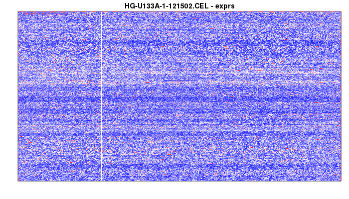
This data is a large matrix (in this case, a 712 by 712 matrix well intensities in the microarray. The image isn’t square because I stretched it purely for better website looks).
Here’s the first six probe ids:
> head(unique(probeNames(data)))
[1] "1007_s_at" "1053_at"   "117_at"    "121_at"    "1255_g_at" "1294_at"
Here’s the first six well measurements:
> head(exprs(data))
  HG-U133A-1-121502.CEL
1                 155.3
2               11016.5
3                 153.3
4               11435.8
5                 114.5
6                 161.3
Let’s also make some graphs about the distribution of well measurements:
> hist(exprs(data))
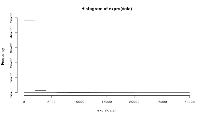
Yep, that’s not useful, let’s try again.
> hist(log(exprs(data)))
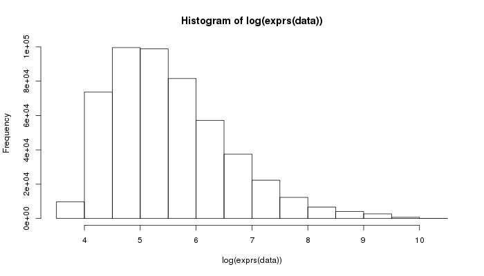
Okay, log-intensity seems more useful.
So this all is pretty neat, but what we have is a matrix of all sorts of different intensity measurements when what we want is normalized expression values for each probe id and, ultimately, each gene.
Normalization, first pass!
As I mentioned last time, there’s all sorts of reasons for why the collected dataset is full of noise, including but not limited to:
- bonding affected by temperature
- small molecules or other impurities in the RNA measurement medium
- variations in quality control of the probes, the microarray, the fluorescent dye, or the sample being measured
- tighter binding between C and G base pairs than A and T
- man who even knows what else, this isn’t digital
- in fact holy cow what if your grad student doing the measurement is mostly thinking about the latest episode of Empire and isn’t paying attention? Whoops you’re actually measuring saliva now.
- moving into caves is sounding pretty good, we could grow mushrooms and stuff come join me it’d be sweet.
- Mmmm sautéed mushrooms.
- butter
- mushrooms
- melt butter in a large skillet where was I?
To deal with all this noise, there’s a number of different strategies used for turning the data into something useful. A lot of smart people have thought about this way longer than I have and come up with some really strong strategies. In fact, the default Affymetrix software that comes with that manufacturer’s microarrays takes care of the first pass of some of this normalization for you.
I don’t have a copy of Affymetrix software, but the authors of the
affy library have attempted to duplicate one of their
normalization techniques for mismatch-based microarrays. We’ll run
it now:
> expressionset <- mas5(data)
background correction: mas
PM/MM correction : mas
expression values: mas
background correcting...done.
22283 ids to be processed
|                    |
|####################|
>
And the first six probe id expressions:
> head(exprs(expressionset))
          HG-U133A-1-121502.CEL
1007_s_at             999.06146
1053_at               949.14361
117_at                 49.40164
121_at               1016.47743
1255_g_at              28.89920
1294_at               148.71909
>
Yay! Except we’re not going to use this. mas5 is fine, but
the following excerpt from the affy documentation is admittedly
worrisome:
The methods used by this function were implemented based upon available documentation. In particular a useful reference is Statistical Algorithms Description Document by Affymetrix. Our implementation is based on what is written in the documentation and, as you might appreciate, there are places where the documentation is less than clear. This function does not give exactly the same results. All source code of our implementation is available. You are free to read it and suggest fixes.
Oh, don’t worry, author of the affy library, I definitely
appreciate that!
Instead of using this technique, researchers often use one of a number of other techniques. One of the more common approaches to normalization is what’s called Robust Multi-array Average, or RMA. Essentially, RMA throws out mismatch probes (which is nice for arrays that don’t have them), and instead turns all of the intensity values into quantiles. It considers these quantiles across multiple microarray experiments to better come up with a statistically valid comparison. This is a pretty strong approach, but a downside with it is that if you then want to start comparing yet another microarray dataset, you will need to re-run your RMA normalization.
Tradeoffs about how to clean your data: The Data Science Story.
Probes to genes
Genes, like pretty much everything else in biology, are variable on a number of fronts - one of which is length. Some genes are short and others are long. Microarray probes, on the other hand, are all the same length.
Because of this, probes are chosen to find genes in such a way that there might be multiple probes for any given gene. If all the probes are activated, then the gene is probably there. As a result, in addition to all this normalization, a further data cleaning step will usually involve mapping probe ids to gene ids.
Luckily, Dr. Stephen Piccolo (along with his colleagues including my lab’s PI) has come up with package that will not only read CEL files, account for mismatch probes if they exist, normalize the data in such a way that it is comparable to other, yet-unknown CEL files, but also map it to genes. Yay!
So let’s use SCAN.UPC, the package in question to load our CEL file. We’ll also have to tell it to download a gene list mapping.
> library(SCAN.UPC)
> pkgname <- InstallBrainArrayPackage("HG-U133A-1-121502.CEL", "20.0.0", "hs", "ensg")
> data <- SCAN("HG-U133A-1-121502.CEL", probeSummaryPackage=pkgname)
(Note: as of this writing, InstallBrainArrayPackage does not use https!
Hope your computer is quarantined!)
Let’s check out the data!
> head(exprs(data))
                HG-U133A-1-121502.CEL
AFFX-BioB-3_at              0.2173211
AFFX-BioB-5_at              0.2150827
AFFX-BioB-M_at              0.6611921
AFFX-BioC-3_at              0.7828146
AFFX-BioC-5_at              0.7416731
AFFX-BioDn-3_at             2.1812713
It has data! Unfortunately those AFFX genes are control probe sets.
Let’s look at the other end of the data.
> tail(exprs(data))
                   HG-U133A-1-121502.CEL
ENSG00000280099_at            0.15484421
ENSG00000280109_at            0.16881395
ENSG00000280178_at           -0.19621641
ENSG00000280316_at            0.08622216
ENSG00000280401_at            0.15966256
ENSG00000281205_at           -0.02085352
Alright! Those are Ensembl genes, and we have normalized measurements for their intensity. Success!
> hist(exprs(data))
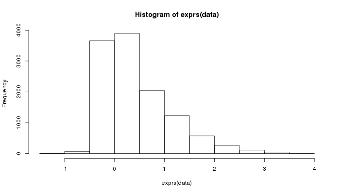
Whew
Alright, stay tuned for where this all gets us, and more importantly, all the corrections I’m going to have to post for this entry!
Update: first blood! Mismatch probes are only on early microarrays. Later Affymetrix microarrays don’t have mismatch probes at all. My descriptions have been updated to reflect this. I also want to sincerely thank Dr. Piccolo both for his thorough help in helping me understand this stuff, for his excellent SCAN.UPC library, and for proof-reading this post!